ML - 06. MLP 코드구현(회귀)

ML - 06. MLP 코드구현(회귀)

import numpy as np

def weighted_sum(x, w, b):
    return np.sum(x * w, axis = 1) + b

#sigmoid activate function
def sigmoid(x):
    return 1 / (1 + np.exp(-x))
def sigmoid_dif(x):
    return sigmoid(x) * (1-sigmoid(x))

#실제 결과로 매핑할 데이터
train_x = np.array([ [1, 1, 0, 1, 0, 1, 1, 0, 1, 1, 0, 1, 1, 1, 1]# 0
                    ,[0, 1, 1, 1, 0, 1, 1, 0, 1, 1, 0, 1, 1, 1, 1]# 0
                    ,[1, 1, 1, 1, 0, 0, 1, 0, 1, 1, 0, 1, 1, 1, 1]# 0
                    ,[1, 1, 1, 1, 0, 1, 1, 0, 1, 1, 0, 1, 1, 0, 1]# 0
                    ,[0, 0, 0, 1, 1, 0, 0, 1, 0, 0, 1, 0, 1, 1, 1]# 1
                    ,[0, 1, 0, 0, 1, 0, 0, 1, 0, 0, 1, 0, 1, 1, 1]# 1
                    ,[0, 1, 0, 1, 1, 0, 0, 1, 0, 0, 0, 0, 1, 1, 1]# 1
                    ,[0, 1, 0, 1, 1, 0, 0, 1, 0, 0, 1, 0, 0, 1, 1]# 1
                    ], dtype="uint8")# * 255
train_y = np.array([0, 0, 0, 0, 1, 1, 1, 1], dtype="uint8")

# print(train_x)
# print(train_y)


# input - hidden layer
w1 = np.random.randn(6, 15)
# print("weight1\n", w1)
b1 = np.random.randn(6)
# print("bias1\n", b1)


# hidden - output layer
w2 = np.random.randn(1, 6)
# print("weight2\n", w2)
b2 = np.random.randn(1)
# print("bias2\n", b2)

epoch = 1000
learnRate = 0.7
mse = []
Error = None
for index_epoch in range(epoch):
    print(index_epoch+1, "번째 학습입니다.", index_epoch+1 , "/", epoch)
    err = []
    for index_train in range(len(train_x)):
        # FeedForword(순전파)
        # input to hidden Layer
        i2hLayerNet = weighted_sum(train_x[index_train], w1, b1)
        i2hLayer = sigmoid(i2hLayerNet)
        # hidden to output Layer
        h2oLayerNet = weighted_sum(i2hLayer, w2, b2)
        h2oLayer = sigmoid(h2oLayerNet)

        # Error
        Error = ((train_y[index_train] - h2oLayer)**2)/2
        err.append(Error)

        #Back-Propagation(역전파)
        # Cost = loss function differential * sigmoid differential
        Cost = -(train_y[index_train] - h2oLayer) * sigmoid_dif(h2oLayerNet)

        # hidden to output Layer
        a2 = Cost
        b2 = b2 - learnRate * a2
        w2 = w2 - (learnRate * a2.reshape(a2.shape[0], 1) * i2hLayer)

        # input to hidden Layer
        a1 = np.sum(a2.reshape(a2.shape[0], 1) * sigmoid_dif(i2hLayerNet), axis=0)
        b1 = b1 - learnRate * a1
        w1 = w1 - (learnRate * a1.reshape(a1.shape[0], 1) * train_x[index_train])

    #학습완료
    print("mse", sum(err))


zero = np.array([    1, 1, 1
                    ,1, 0, 1
                    ,1, 0, 1
                    ,1, 0, 1
                    ,1, 1, 1], dtype="uint8")# * 255
one = np.array([    0, 1, 0
                   ,1, 1, 0
                   ,0, 1, 0
                   ,0, 1, 0
                   ,1, 1, 1], dtype="uint8")# * 255
test = [zero, one]
for index in range(len(test)):
    # input to hidden Layer
    i2hLayer = sigmoid(weighted_sum(test[index], w1, b1))

    # hidden to output Layer
    h2oLayer = sigmoid(weighted_sum(i2hLayer, w2, b2))

    #소숫접3이하 버리기
    np.set_printoptions(formatter={'float_kind': lambda x: "{0:0.3f}".format(x)})
    print(h2oLayer)

 

구조

trainData

왼쪽 정상건에 비해 노이즈가 낀 train데이터 생성

#실제 결과로 매핑할 데이터
train_x = np.array([ [1, 1, 0, 1, 0, 1, 1, 0, 1, 1, 0, 1, 1, 1, 1]# 0
                    ,[0, 1, 1, 1, 0, 1, 1, 0, 1, 1, 0, 1, 1, 1, 1]# 0
                    ,[1, 1, 1, 1, 0, 0, 1, 0, 1, 1, 0, 1, 1, 1, 1]# 0
                    ,[1, 1, 1, 1, 0, 1, 1, 0, 1, 1, 0, 1, 1, 0, 1]# 0
                    ,[0, 0, 0, 1, 1, 0, 0, 1, 0, 0, 1, 0, 1, 1, 1]# 1
                    ,[0, 1, 0, 0, 1, 0, 0, 1, 0, 0, 1, 0, 1, 1, 1]# 1
                    ,[0, 1, 0, 1, 1, 0, 0, 1, 0, 0, 0, 0, 1, 1, 1]# 1
                    ,[0, 1, 0, 1, 1, 0, 0, 1, 0, 0, 1, 0, 0, 1, 1]# 1
                    ], dtype="uint8")# * 255
train_y = np.array([0, 0, 0, 0, 1, 1, 1, 1], dtype="uint8")

---

Layer

# input - hidden layer
w1 = np.random.randn(6, 15)
# print("weight1\n", w1)
b1 = np.random.randn(6)
# print("bias1\n", b1)


# hidden - output layer
w2 = np.random.randn(1, 6)
# print("weight2\n", w2)
b2 = np.random.randn(1)
# print("bias2\n", b2)

---

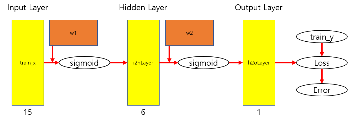
feedforword

# FeedForword(순전파)
# input to hidden Layer
i2hLayerNet = weighted_sum(train_x[index_train], w1, b1)
i2hLayer = sigmoid(i2hLayerNet)
# hidden to output Layer
h2oLayerNet = weighted_sum(i2hLayer, w2, b2)
h2oLayer = sigmoid(h2oLayerNet)

---

backpropagation

#Back-Propagation(역전파)
# Cost = loss function differential * sigmoid differential
Cost = -(train_y[index_train] - h2oLayer) * sigmoid_dif(h2oLayerNet)

# hidden to output Layer
a2 = Cost
b2 = b2 - learnRate * a2
w2 = w2 - (learnRate * a2.reshape(a2.shape[0], 1) * i2hLayer)

# input to hidden Layer
a1 = np.sum(a2.reshape(a2.shape[0], 1) * sigmoid_dif(i2hLayerNet), axis=0)
b1 = b1 - learnRate * a1
w1 = w1 - (learnRate * a1.reshape(a1.shape[0], 1) * train_x[index_train])

테스트결과

[0.016] 정답레이블 : 0
[0.994] 정답레이블 : 1

 

위의 예시처럼 회귀는 연속적인 숫자중 하나로 출력됨

하지만 2개로 분류할수 있는 경우라면 반올림을 통해 이진분류로 사용할 수 있음